What’s this blog about?
In this blog, I’ll be sharing one of the assignments I did in my parallel programming course, taught by the great Professor Xu Weizhong of CUHK-SZ. This blog will be divided into three parts: what the assignment was about, what I was taught in class to make my code run faster, and what I did to further optimize my code to ultimately make it run 9x faster.
BTW, the code can be seen on my GitHub repo (although I literally just upload what I submitted as my assignment lol)
Part I: Bilateral Filter - an embarrassingly parallel assignment
Do you know how a program blurs images? If you do, then good for you.
If you don’t, well it’s quite simple. A program will have a kernel of size MxN (M is usually equal to N). The program will then start by laying the kernel at the top left corner of the image. Then, for every pixel that overlaps with the kernel, the program will change its value to the average pixel value of all pixels that overlap with the kernel. Once completed, the program will move on by moving right or down, until all sections have been blurred.
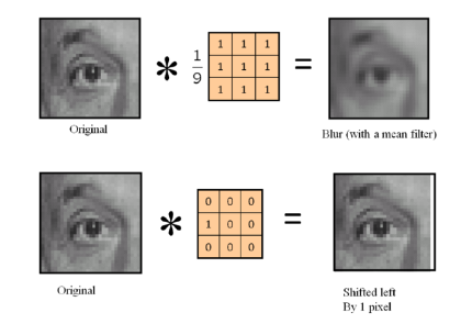 Image from naver.com
Well, Bilateral filter is just like that!
However, the key difference is, instead of just simply averaging the pixel values, each individual pixel will have its value adjusted based on their relative position on the kernel. More specifically, the value of each individual pixel can be expressed as:
$$ I’(p) = \frac{1}{W_p} \sum_{q \in \Omega} I(p) * k_r\left(\left| I(q) - I(p) \right|\right) * k_s\left(\left| q - p \right|\right) $$
For normalization term $W_p$:
$$ W_p = \sum_{q \in \Omega} k_r\left(\left| I(q) - I(p) \right|\right) * k_s\left(\left| q - p \right|\right) $$
Where:
- $I$ is the image intensity
- $p$ and $q$ are pixel positions
- $\Omega$ is the kernel window
- $k_r$ and $k_s$ are the range and spatial kernels
With: $$ k_r(p) = \exp\left(-\frac{\left| p \right|^2}{2\sigma_r^2}\right), \quad k_s(p) = \exp\left(-\frac{\left| p \right|^2}{2\sigma_s^2}\right) $$
Part II: Vector registers - how knowing your CPU architecture can make your code run faster
Suppose we have two array of integers, a and b. For each index i, we want to add the element of a with b, and we store it on the i-th index of the array c. How do we do that?
Well, one way is to use for loop to traverse each index one by one:
#include <iostream>
using namespace std;

int main(){
    int a[2] = {1, 2};
    int b[2] = {3, 4};
    int c[2];

    for (int i = 0; i<2; i++){
        c[i] = a[i] + b[i];
    }

    return 0;
}
However, this method is very slow since we add the numbers one by one (i.e. sequentially). Is there a better way? Can we add multiple elements at once?
Well turns out there is a way.
Enter SIMD (Single Instruction Multiple Data) paradigm: in modern CPUs, there is a set of special registers known as vector registers. What makes these registers special is that, unlike the regular registers, operations on vector registers are done in parallel because the data on these registers are processed by a special ALU, known as vector ALU.
Below is an illustration on how data on both types of registers are processed (let’s use 4 bits for simplicity):
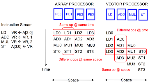
TL;DR: data in normal registers are processed sequentially. vector registers are processed in parallel.
Let’s get back to the Bilateral filter problem. We have the following equations:
$$ I’(p) = \frac{1}{W_p} \sum_{q \in \Omega} I(p) * k_r\left(\left| I(q) - I(p) \right|\right) * k_s\left(\left| q - p \right|\right) $$
$$ W_p = \sum_{q \in \Omega} k_r\left(\left| I(q) - I(p) \right|\right) * k_s\left(\left| q - p \right|\right) $$
$$ k_r(p) = \exp\left(-\frac{\left| p \right|^2}{2\sigma_r^2}\right), \quad k_s(p) = \exp\left(-\frac{\left| p \right|^2}{2\sigma_s^2}\right) $$
From here, we can see that $I’(p)$ of a pixel doesn’t depend on the $I’(p)$ of another pixel. Therefore, we can very easily parallelize our program.
OK. But how do we write a program that uses this so-called vector registers?
Well, it depends on your specific CPU, but if yours is Intel, then you can use AVX intrinsics. To use it, you first need to load your data into the vector registers using load commands. One example is _mm256_set_ps(), which loads data to a vector register of size 256 bits. If your data is less than 256 bits, then you need to pad it.
Once loaded, you can perform various operations such as arithmetic or bitwise operations. You can check the manual on Intel’s website. You may feel that intrinsics are similar to the Assembly language.
Lastly, once you’re done with the computations, you can unload the result using store commands. One example is _mm256_storeu_ps().
Part III: Taylor Series - how I used approximation to optimize my code
OK. Now that our program runs in parallel, we should be done, right?
Well, not so fast. You see, while SIMD is a powerful concept on paper, in reality, it is very limited in what it can do: for Intel’s intrinsics, we can only perform basic arithmetic and bitwise operations such as addition, multiplication, bitwise or, etc.
Let’s get back to our bilateral filter formulas. Two of them are:
$$ k_r(p) = \exp\left(-\frac{\left| p \right|^2}{2\sigma_r^2}\right), \quad k_s(p) = \exp\left(-\frac{\left| p \right|^2}{2\sigma_s^2}\right) $$
Which requires doing exponent operations. However, there is no instructions that can do this in Intel’s intrinsics. To solve this, the easy and dirty approach is as follows:
- load the data to
vector registers - do computations using the
SIMDparadigm - when we reach the point where we have to do exponent operations, we first unload our results to
normal registers - do exponent operations the traditional way
- load the data back to
vector registers - do the remaining computations using the
SIMDparadigm - unload our results to
normal registersone last time
This method works. But can we do better? Can we do the entire computation of the Bilateral filtering in SIMD?
Well, to find the answer, let’s move on to a different problem, one we may find from high school.
Let’s say you’re in your high school’s lab doing an experiment and you plot the results of your experiment. You may come up with something like this (yes I know there are no labels, but they are not important):
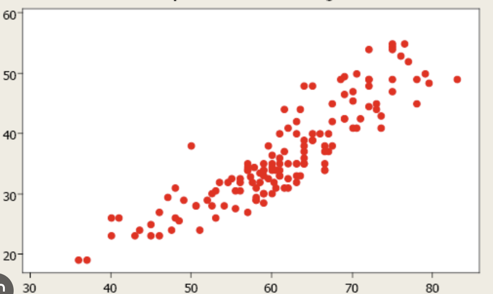
Now, you may want to find a relationship between the y axis and x axis. Through visual inspection, you may find a line that best describes the relationship between the two, the best-fit line (which is a first-order polynomial):
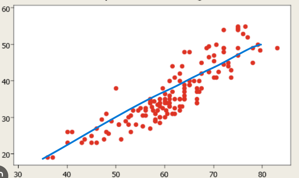
This raises two questions:
- Is there a more rigorous procedure (not visual inspection) to approximate a function (relationship)?
- Can we do better than “best-fit line”? Can we do “best-fit quadratic” (second-order polynomial)? “best-fit quartic” (third order)?
Enter the Taylor Series. The Taylor Series can be mathematically described as:
$$
f(x) = \sum_{n=0}^{\infty} \frac{f^{(n)}(a)}{n!} (x - a)^n
$$
What is this? Well, essentially, Taylor Series is a polynomial approximation of a function $f(x)$ and we can decide the degree of the polynomial by changing the value of n.
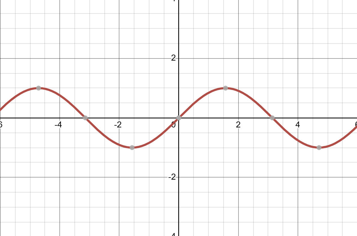
I think it would be best to use real example. Consider the function $f(x) = sin(x)$. The function looks like:
Now let’s approximate it using the Taylor series. When n = 1:
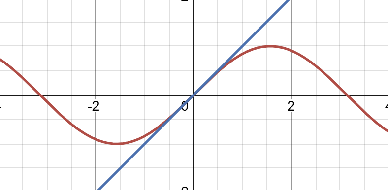
This is our best-fit line for the function $f(x) = sin(x)$, centered at $x = 0$. Moving on, let’s try n = 3:
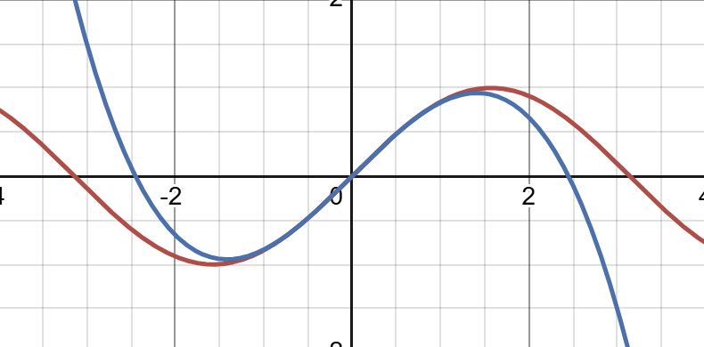
This is now our best-fit quartic. You can see that it resembles the original function better. What about n = 5?
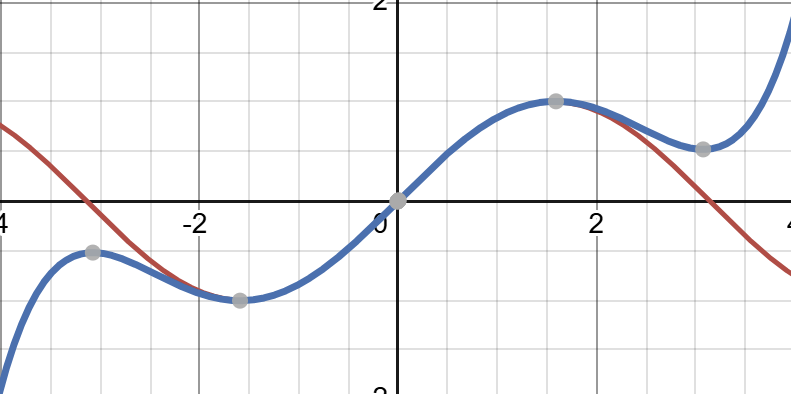
Even better!
This is the power of Taylor Series.
OK, that’s cool. But how does it help with our Bilateral filter program?
Well, remember that Taylor Series gives a polynomial approximation to a given function. What’s so special with polynomials? They can be computed using basic arithmetic operations, namely addition, subtraction, multiplication, and division - operations that can be done in Intel’s vector intrinsics!
And that’s what I did: I approximated the exponent operations using the Taylor Series. For my case, I used n = 5.
Results & conclusion
After all is said and done, here’s the result: my code took 371 ms to run, far faster than the teaching team’s own implementation at 3674 ms; nearly 10x as fast.
I remember during lectures, Professor Xu kept on saying “Vector is the future.”. Early on, when I first heard him repeating that phrase in class, I told to myself, “Damn, this guy is an extremist. How can he be so sure?”. Well, after doing the assignment, I felt like I understand his point.
Well, that’s all for now. As mentioned early in this blog, you can find my code on my GitHub (although I only shared the one I submitted, so you need to do modifications in order for it to run).