What’s this blog about?
This is the second part of Creating Neural Networks: Concepts, Math, and Code, where we will be creating a neural network from scratch. If you don’t have a prior knowledge on the concepts of neural networks, then please read part I before you read this article.
BTW, all the codes are available on my GitHub repo.
Lastly, this is a blog I wrote at Medium.com back in 2023 when my writing skills were worse; so you may find it too wordy.
Planning
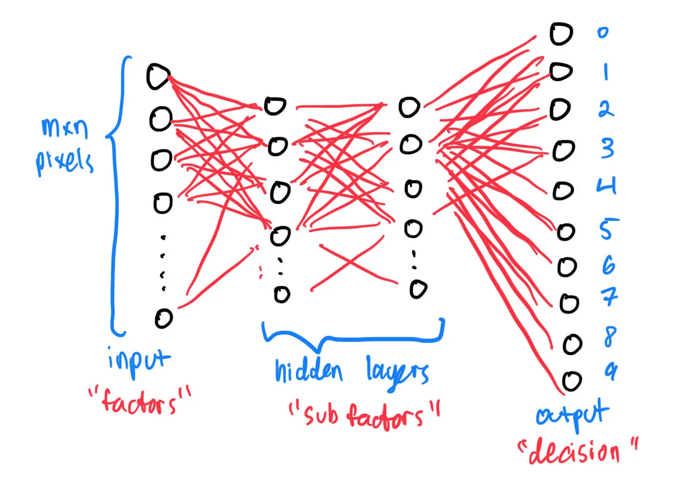
Before we begin, let us first plan how we want to implement the code. For this article, we’ll create one with modular layers, so we can experiment with various network configurations (architecture). Below is a diagram on how our neural net might look like:
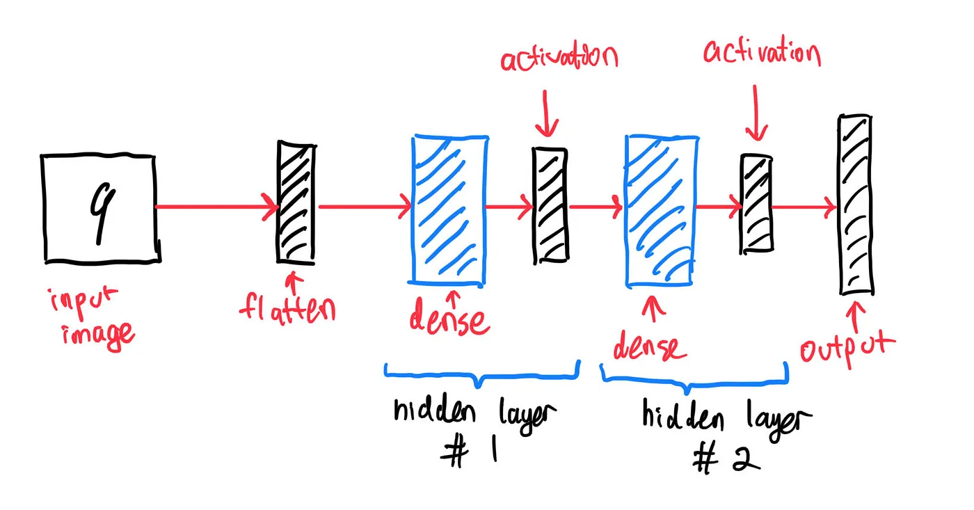
For our input image, we will use the MNIST handwritten digits dataset, where each input image is a picture of size 28x28 pixels. Without further ado, let’s begin by creating the code for each type of layers.
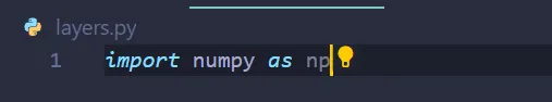
Create a file named layers.py and import the NumPy module:
Layer: Flatten
What does the layer flatten do? Well, in order for us to process the 28x28 image in our neural net, we first need to flatten it into 784x1 input pixels.
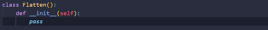
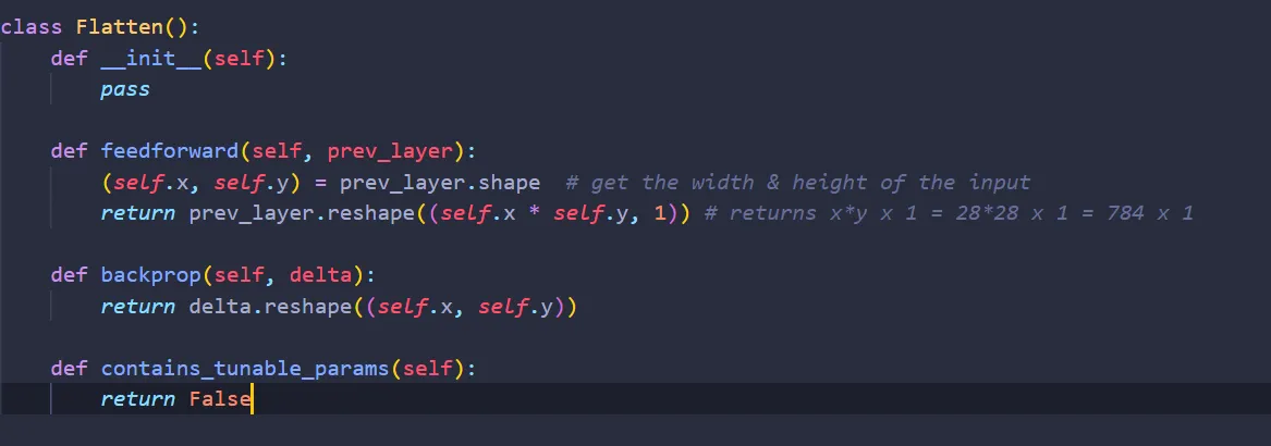
Let’s begin by creating a class called Flatten:
Feedforward
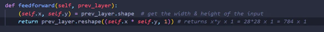
When Flatten receives an input called prev_layer, its job is to flatten it into a 28x28 pixels. We can do that easily with NumPy:
Backpropagation
Now, what happens when we get delta, the partial derivative of our error function with respect to the next layer? Well, for Flatten, we simply reshape vector from 784x1 to a 28x28 matrix:

That’s all! One question: does Flatten contains any weights or biases that we need to tune? No! Let’s add that to the class Flatten:

Why would we need to add this function? Well, it will come in handy later. All in all, here’s the complete code for the class Flatten:
Layer: Dense
Here comes the fun part: the dense layer. What does the dense layer do, actually? Well, remember this diagram?
Let’s focus on one layer:
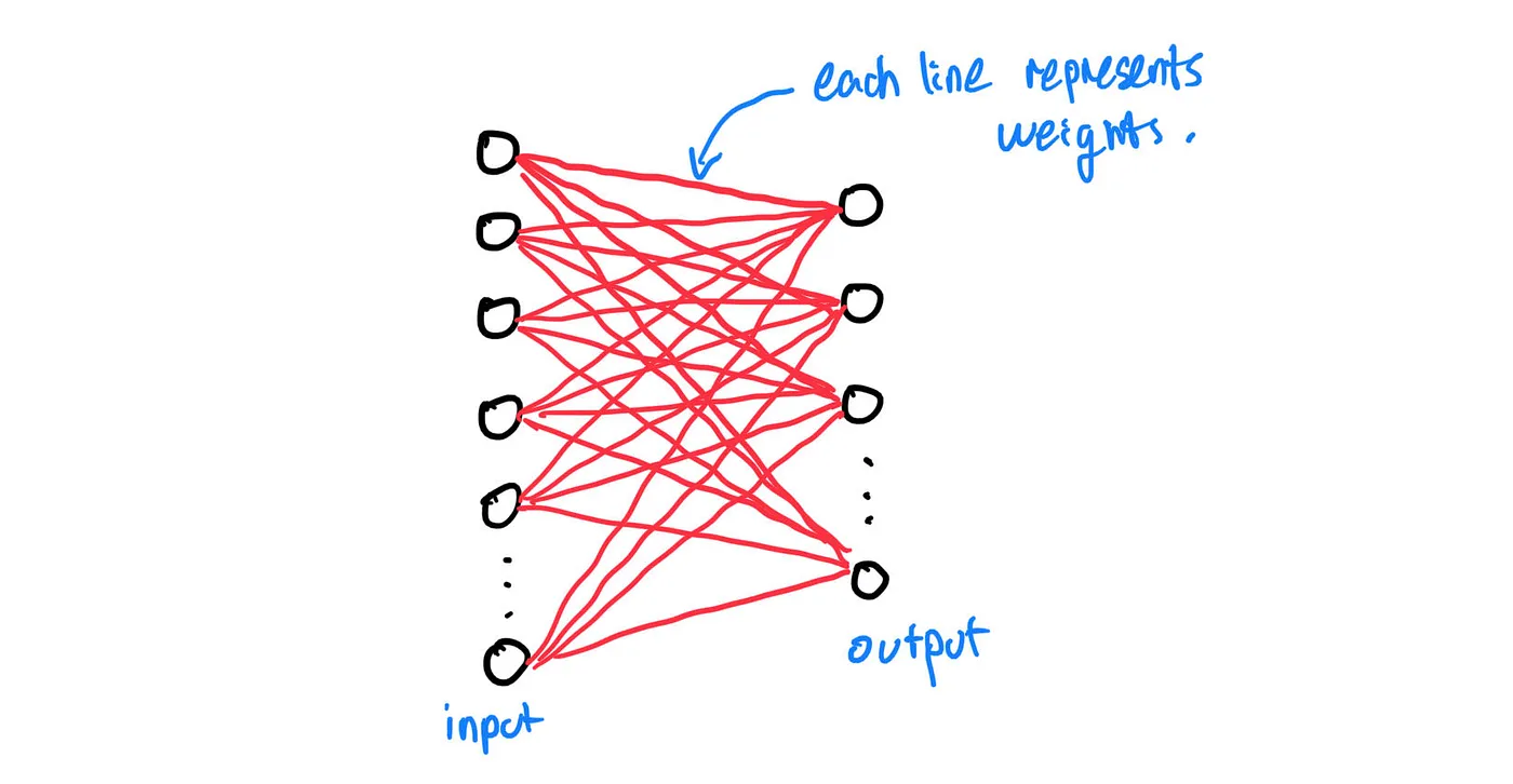
Essentially, each input node will have its value being multiplied by a weight (represented by a line) before being fed into an output node. We repeat this process until that input node has been connected to all the output nodes:
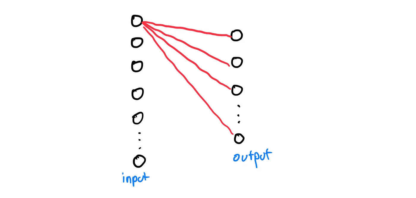
Lastly, when we have repeated the process mentioned in the previous paragraph to all input nodes, each output nodes will add all the weighted input nodes together before finally adding a bias:
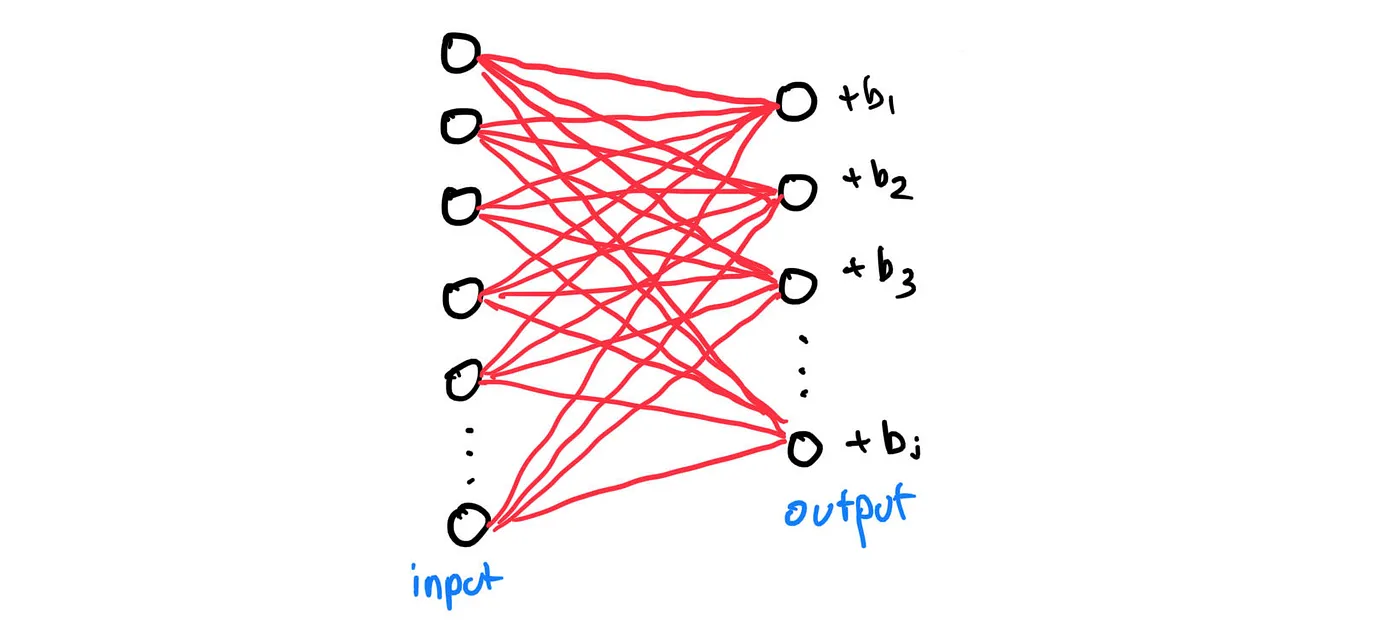
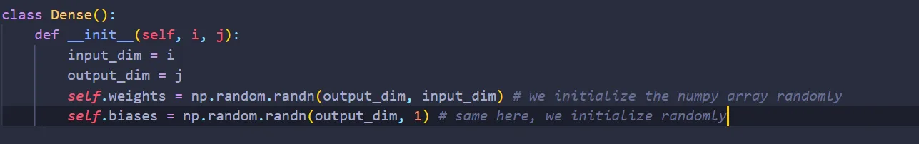
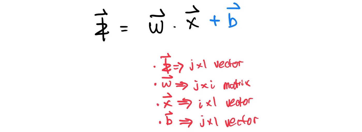
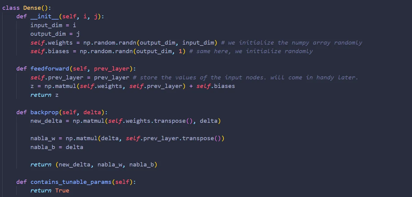
Now, what can we do? well, suppose that there are i input nodes and j output nodes. We can represent the weights as a matrix of size j x i and the biases as a vector of size j x 1. With that, let’s create the class Dense:
Feedforward
Alright. Now, what do we do once we received the input nodes of size i x 1? Well, we multiply them by the weights. Mathematically,
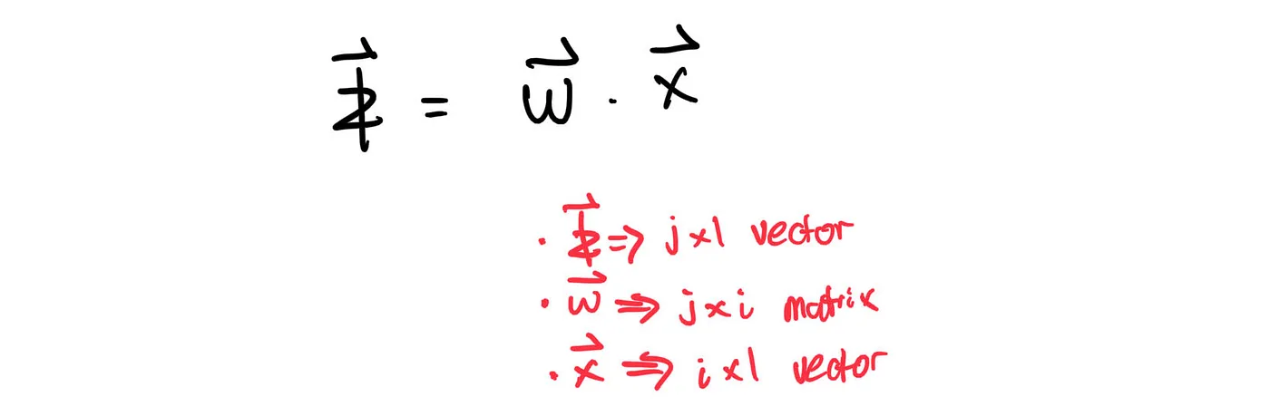
Don’t forget to add the biases:
Translating the above equation into code, we get:
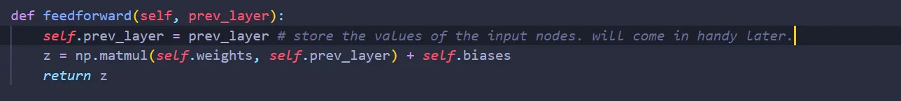
By the way, I am storing the values of the input nodes. It will come in handy shortly.
Backpropagation
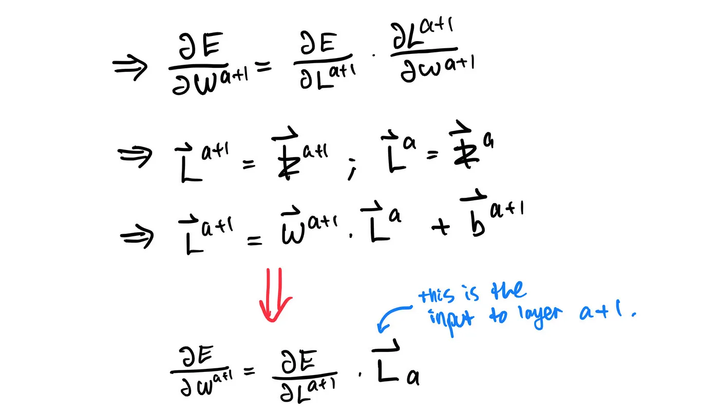
We ended part I with the equation:

The partial derivate of the error function with respect to layer a+1 is easy — it’s delta. But how does layer a+1 relate to layer a?
one key observation here is the output of a layer is the input of the layer right after it. Well, let’s focus on the first node at layer a.
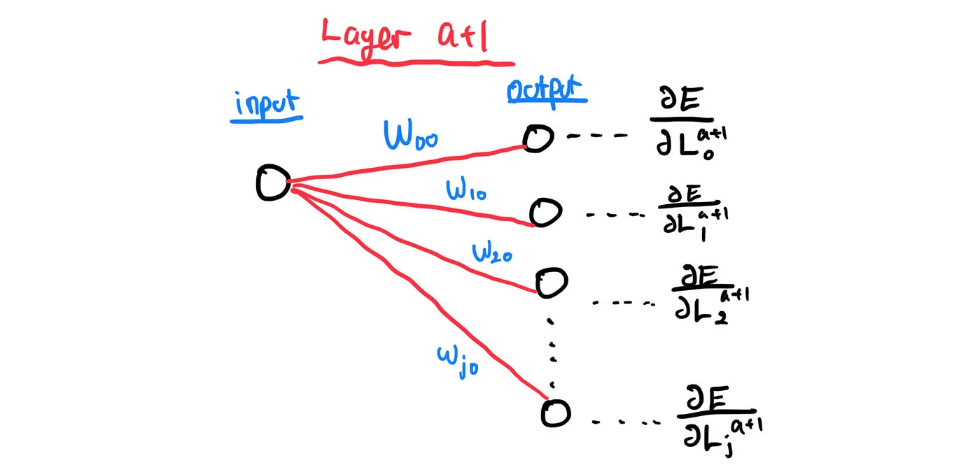
Mathematically, we can express what happened above as:
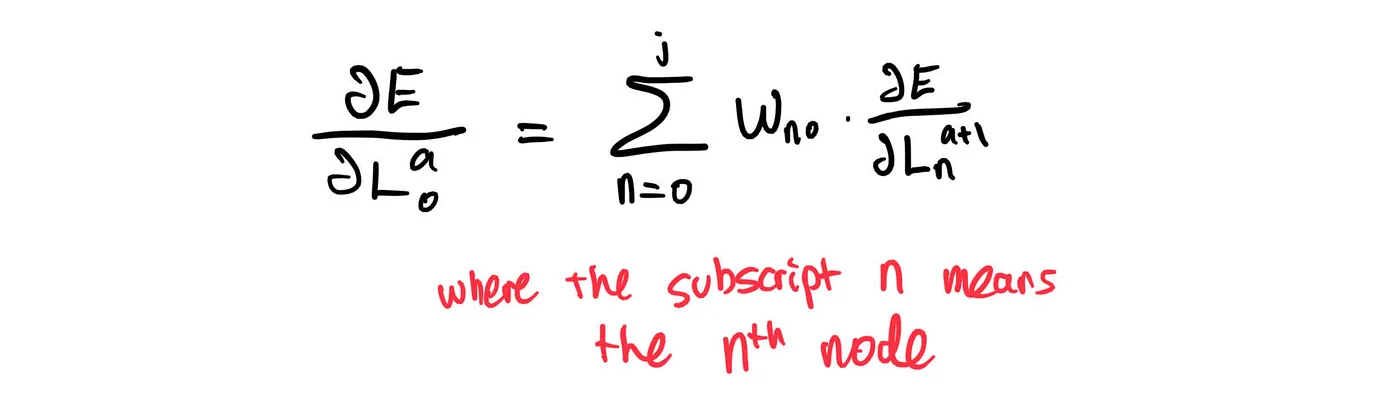
To generalize,

We can make the above equation more compact by expressing it as:

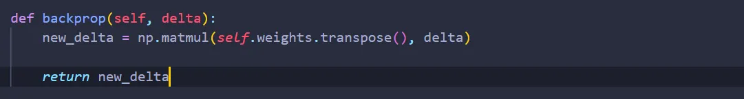
So, during backpropagation, we will receive delta, the partial derivative of the error function with respect to layer a+1 calculated by the layer a+2. In return, layer a+1 will give new_delta, the partial derivative of the error function with respect to layer a for, well, layer a.
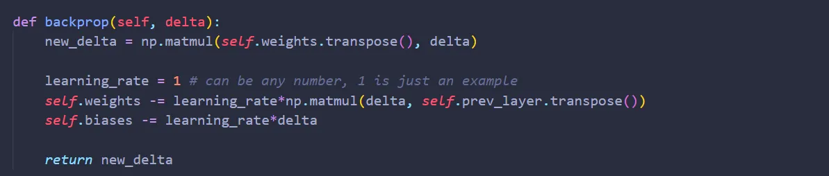
Writing it into code:
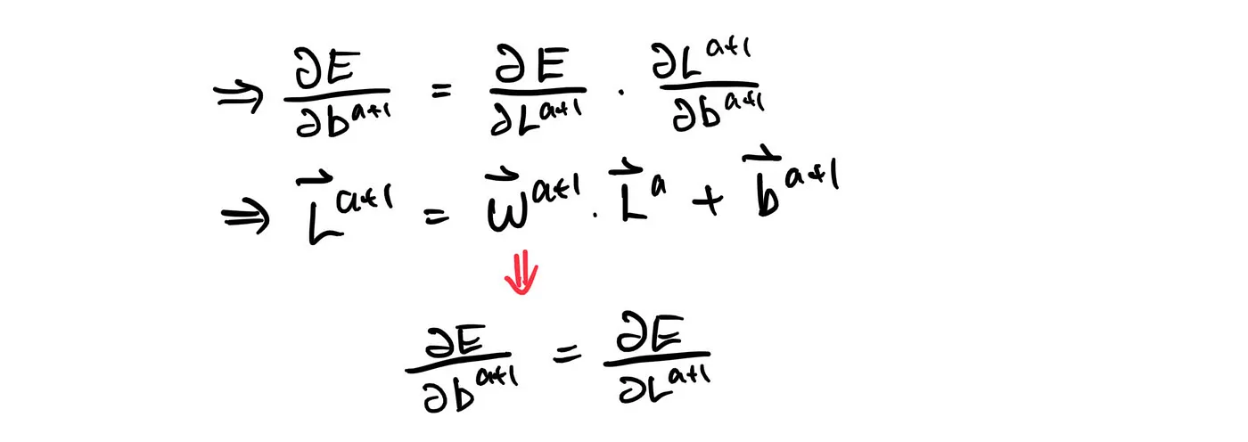
That’s it! Are we done now? Well, not yet. Unlike the layer Flatten, Dense has two tunable parameters: weights and biases. We can perform gradient descent easily. The partial derivative of the error function with respect to the weight is:
For the biases:
given learning rate gamma, the equations for gradient descent then becomes:

Translating them into code,
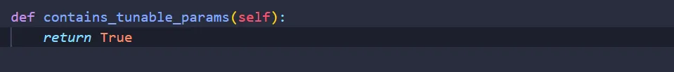
Just like the Flatten class, we also want to add the function contains_tunable_params here as well:
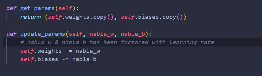
At this point, we are done! However, this code is too rigid — we can only perform gradient descent here. If we want to give the code more flexibility, we can instead return the partial derivatives of error function with respect to the weights and biases, nabla_w & nabla_b, along with new_delta.
My idea here is, instead of letting the class Dense tune its weights & biases by itself, we will create another function that does the tuning. The function can be anything: it can be a gradient descent function, stochastic gradient descent function, etc. However, in order to do that, the class Dense needs to give that function nabla_w & nabla_b; which is why we return those values when backprop is being called.
Since we want to tune the weights & biases from this “mysterious” function, we need to create two functions inside the class Dense that enables this “mysterious” function to access & update the weights.
And now we are done! Here’s how the class Dense looks like:

Layer: Activation
Lastly, we want to add the activation layer. Let’s create a new Python file activations.py and import NumPy again:
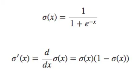
As mentioned in part I, one common activation function is the sigmoid function:
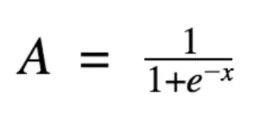
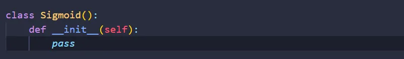
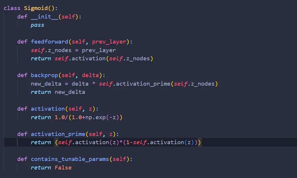
In this article, we will be using Sigmoid as our activation function. First, we create the class Sigmoid:
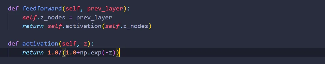
Feedforward
This one is easy. Translating the equation for Sigmoid into code:
Backpropagation
This one is not as easy, but still doable. Let’s use the chain rule again:
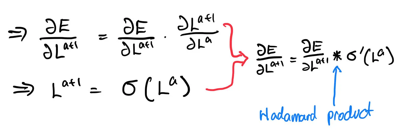
Where the derivative of the sigmoid is:
Translating the above equation into code,
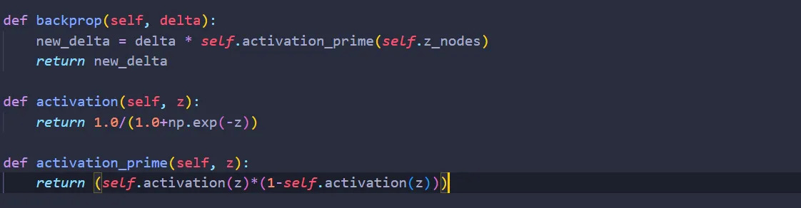
Lastly, since the activation layer doesn’t contain any weights & biases,

We are done! Here’s the finished code:
Putting it all together
Now let’s put it all together. Create a Python file called MLP.py (MLP stands for Multi Layer Perceptron, a type of neural network we can build with what we already have).
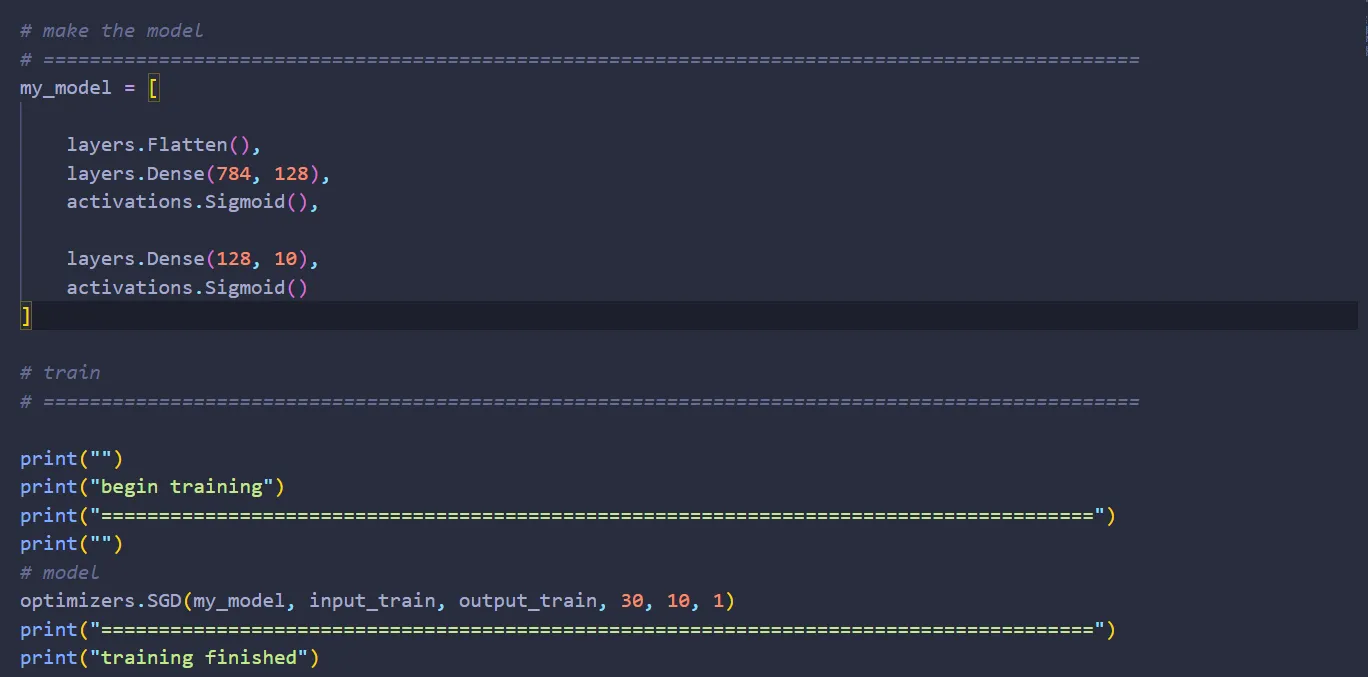
Let’s build a network with one hidden layer with 128 nodes:
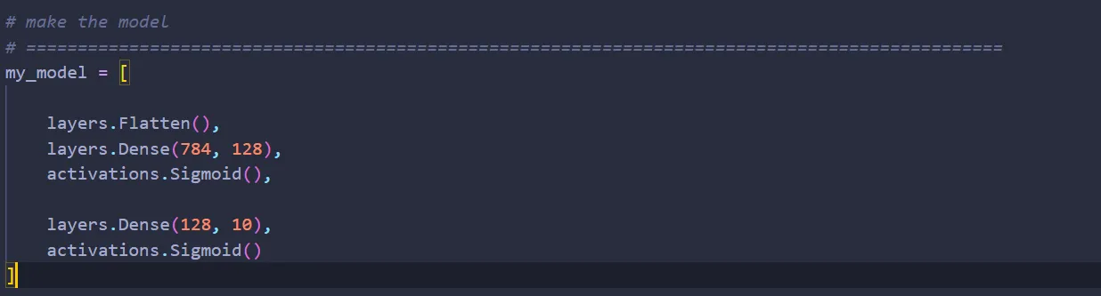
And that’s it! You’ve just built a simple neural network from scratch. There are two problems, though: how do you train it? How do you test it? Let’s tackle these problems one at a time.
Training: Stochastic Gradient Descent
Remember the “mysterious” function we talked about when building the Dense layer? Well, that “mysterious” function can be any function, as long as it tunes the weights & biases of the neural net. In this article, I will be using the stochastic gradient descent, or SGD for short.
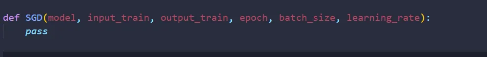
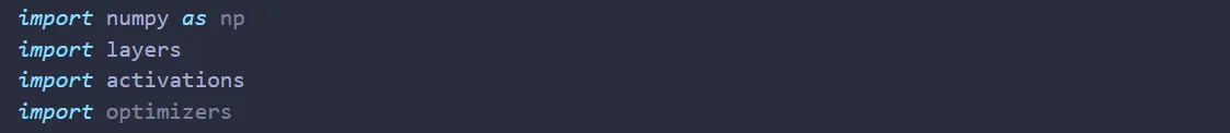
To begin, create another Python file called optimizers.py and import the following modules:

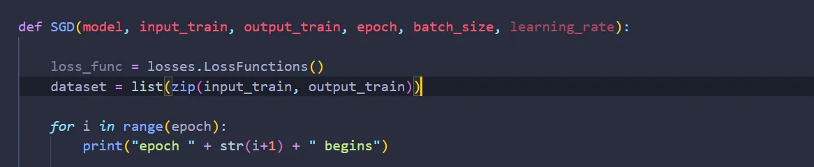
Let’s create a function called SGD. Since this function is used to train our network, we need to give it a reference to our neural network model. We also need to give it the training data, divided into input data and output data, our desired learning rate, the batch size, as well as how many times we want to repeat training the network on the training data we provide (epoch):
Let’s first begin by combining our input & output training data. To do that,
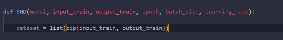
input_train is a list of 50.000 28x28 NumPy array, while output_train is a list of 50.000 10x1 NumPy array in one-hot encoding.
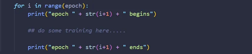
Epoch is the number of times we want to train the network on the training data we provide. To do that, we create a for loop:
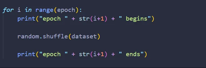
Before we begin, it would be a great idea to shuffle our training data on each epoch, so the ordering of the training data is not the same from one epoch to another:
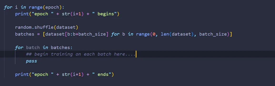
In SGD, we want to feed the network with multiple training data, then we average the error — train the network in batches, so to speak. So, let’s split our training dataset into batches, and train on each separate batch:
As mentioned before, we want to average the error of the network made in a single batch. To do that, we need to keep track of the sum of nabla_w & nabla_b of each layers that contains weights & biases. Let’s create a list of NumPy arrays to store these information:
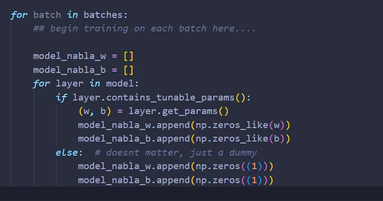
Basically, what the code above means is: If the layer has weights & biases, then to keep track of the sum of nabla_w & nabla_b, create NumPy arrays with the shapes of the weights & biases of that layer, and set the value of each index to zero. Otherwise, just create a NumPy array of size 1. Why size 1? Actually, it doesn’t matter what the shape of the NumPy array is, since we are only using it as a dummy.
If you are confused as to why a dummy needs to be created whenever we have a layer that doesn’t have any tunable parameters, just keep reading; I hope it becomes clear later when we arrive at the part where we want to adjust the weights & biases of each layer.
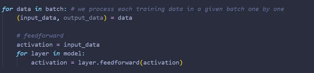
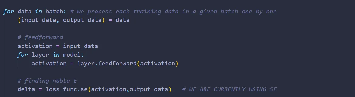
Feedforward Each input training data is the input of the first layer. From that point on, the output of the previous layer will be the input of the current layer; and so on until we reach the final layer.
The output of the final layer is the network’s prediction on what the number written on the image is.
Translating everything into code,
Once the network made its prediction, we compare the prediction with the actual answer, output_data, to obtain the error and ultimately nabla E mentioned in part I.
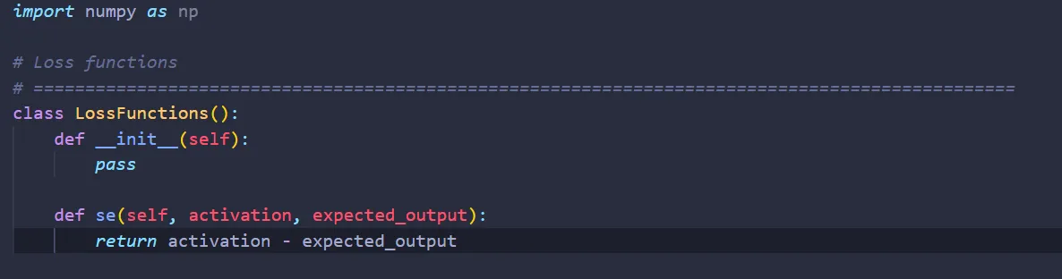
To maintain code modularity, let’s create the function to compute nabla E on a separate Python file called losses.py. Here is the code for losses.py:
Now, we need to import losses.py into optimizers.py:

And create an instance of the class LossFunctions inside the function SGD
Now, we can obtain nabla E by calling loss_func.se() (se means squared error):
Next we do backpropagation, adding nabla_w & nabla_b of each layer to model_nabla_w & model_nabla_b that corresponds to that layer.
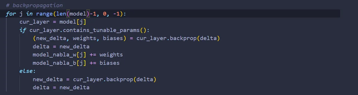
I hope that by now it becomes clear why dummies are needed: We have five layers, three that don’t contain tunable parameters, and two that contain tunable parameters. If we don’t add dummies, then when j = 2, both model_nabla_w & model_nabla_b will already be out of bounds.
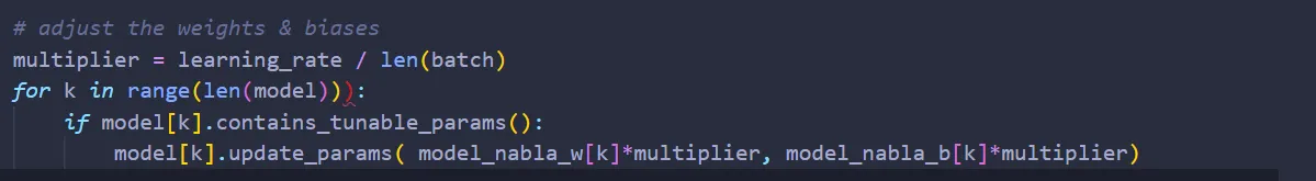
We are almost done. All that’s left to do is to adjust the weights & biases of each layer. But before that, we need to divide the sum of nabla_w & nabla_b with batch_size to obtain the average and multiply them by learning_rate. Only then can we adjust the weights & biases of each layer:
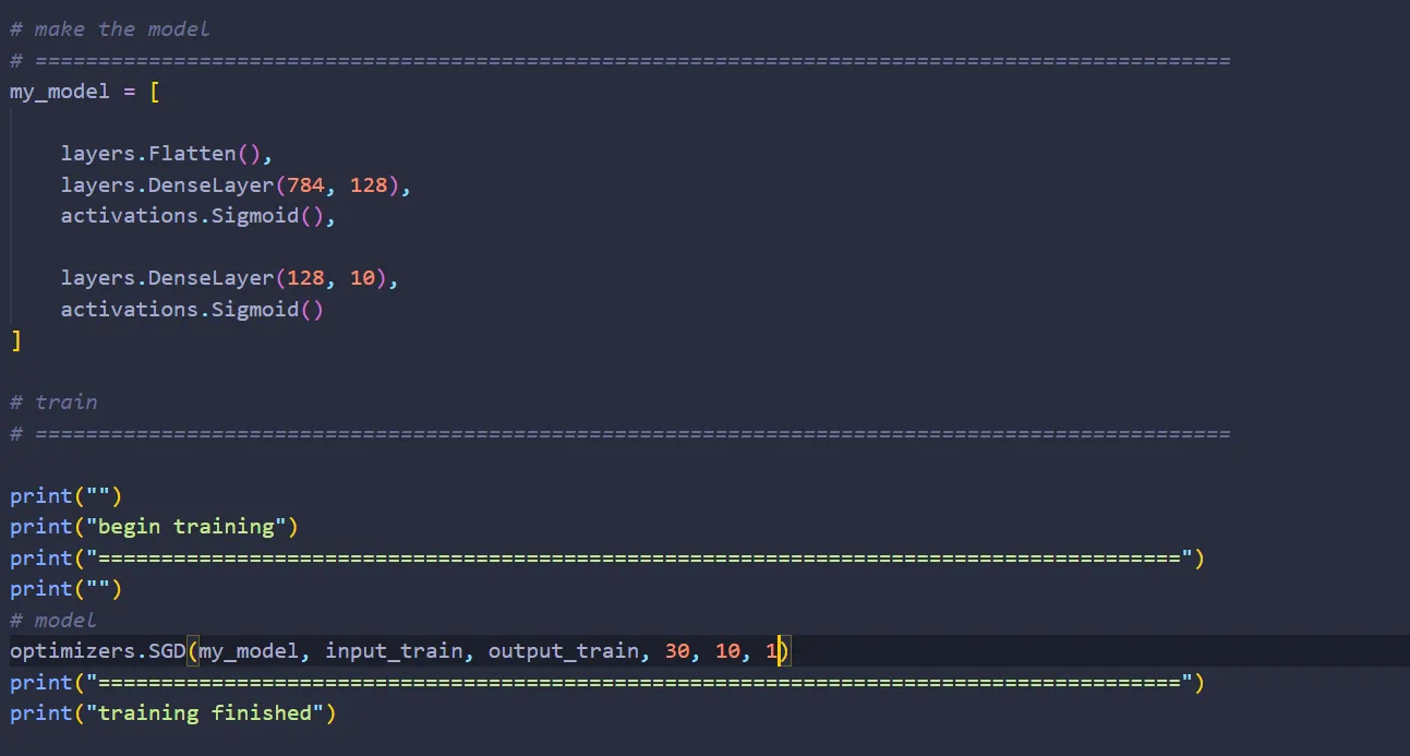
And we are done implementing the SGD! Let’s import optimizers.py onto MLP.py:
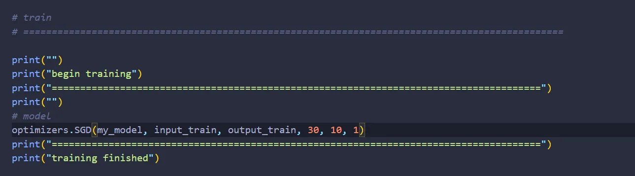
Lastly, let’s train the network:
Now all that’s left to do is to build a function to load the training & test data and another function to test the network.
Loading the data
As mentioned earlier, we will be using the MNIST dataset to test & train our network. Now there are a lot of ways to get the MNIST dataset, but for this tutorial I’ll be using Keras to load the MNIST.
You might be asking, “Aren’t we going to build neural nets from scratch? Why use Keras?”. Well, we did built a neural net from scratch. However, loading data is the least interesting part in building a neural network and frankly, downloading MNIST dataset from other source and load them yourself is not challenging — it’s just tedious.
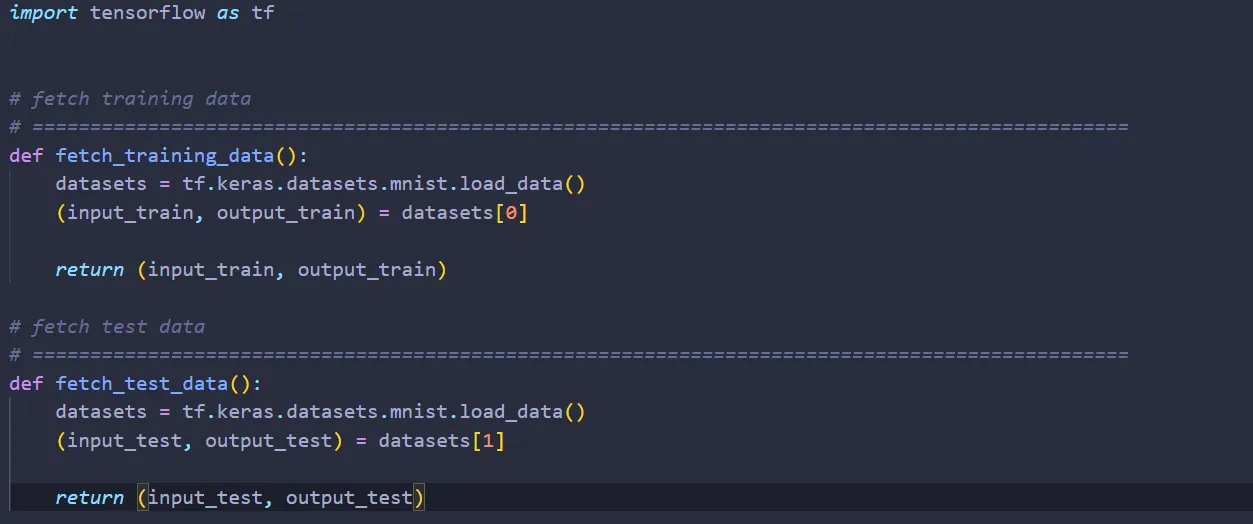
Anyway, let’s create a file called mnist_loader.py and type in the following code:
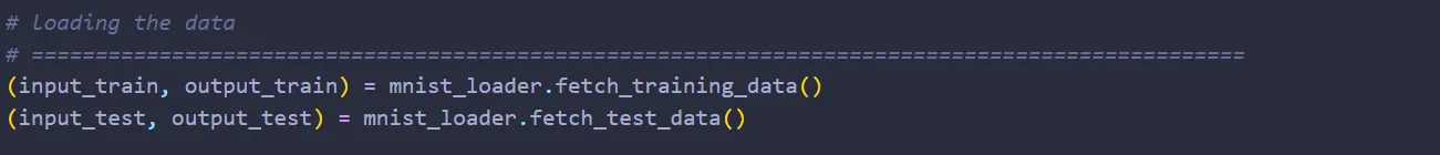
Now, let’s import mnist_loader.py on MLP.py:
Next, fetch the training & test data.
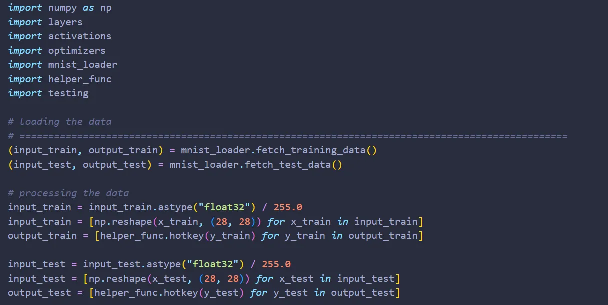
One last thing: we need to process the training & test data before we can use them for training & testing our network.
Let’s start with the input_train. Originally, input_train is a NumPy array of size 50.000x28x28. Let’s convert it to a list of 50.000 NumPy arrays of size 28x28:

Next, the output_train. When we load output_train from Keras, we will be obtaining a NumPy array of size 50.000x1. There are two tasks that we need to do:
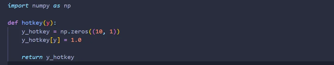
First, output_train must be encoded using the hot-key encoding. To do that, let’s create a file called helper_func.py, which contains, well, a set of helper functions.
Inside helper_func.py, create a function called hotkey:
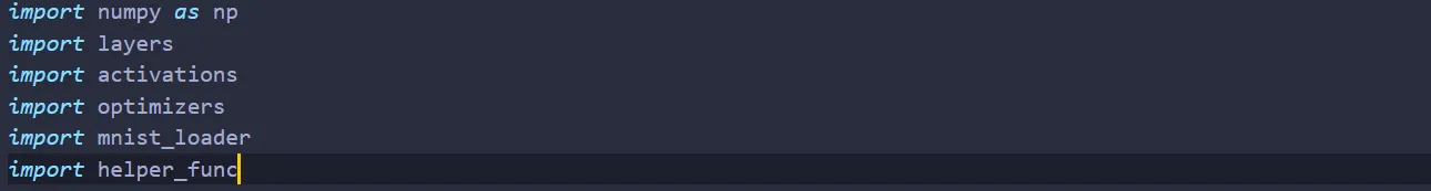
then we import helper_func.py onto MLP.py:
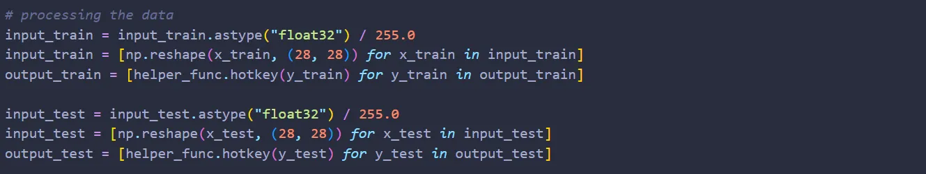
Second, just like input_train, we need to convert the 3-dimensional NumPy array into a list of 2D NumPy arrays. To do that,

Then we repeat for the test data as well. Overall, the code for preprocessing the training & test data looks like:
And we are done with data loading! Kind of tedious, right?
Testing the neural network
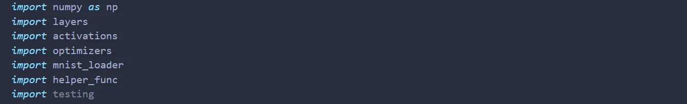
We’re almost done! Let’s now make a Python file testing.py to test our network and import it onto MLP.py:
Inside testing.py, we first import NumPy and helper_func (it will come in handy later).
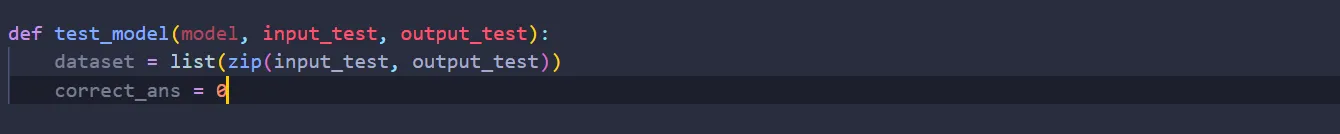
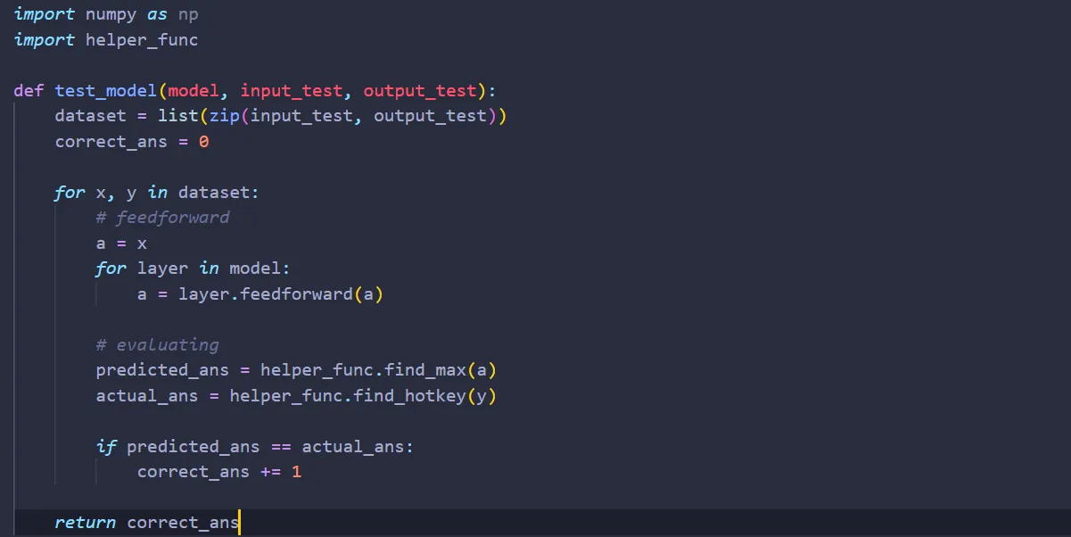
Next, inside testing.py, we create a function called test_model. Just like what we did in optimizers.py, we first combine the input & output data.

Since we are trying to test how often our network guesses correctly, we’ll set a counter:
Now that everything is set, let’s feed our neural network the test data one by one:
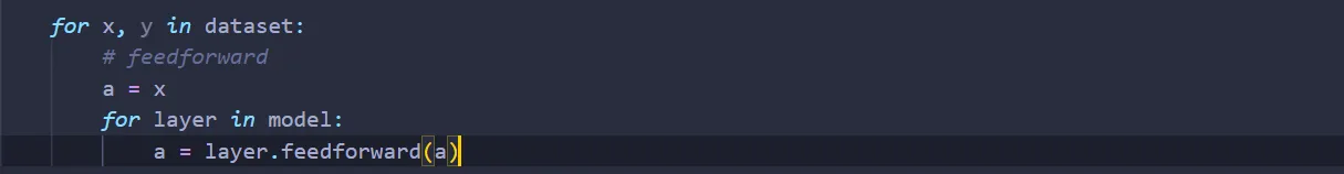
Once we’ve completed the for loop, a will be the prediction the neural net makes for the given input. Now we need to find the output node with the largest value. To do that, let’s create a function called find_max in helper_func.py:
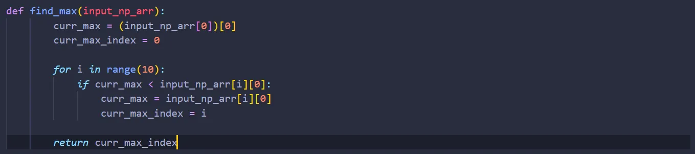
And use it in testing.py:

Now, we need to decode the hotkey encoding of the output, y. To do that, let’s return to helper_func.py once again and create the following function to decode the encoding:
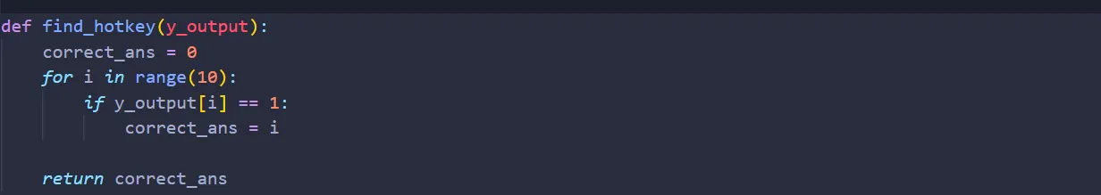
Then, we call the function in testing.py and compare the results:
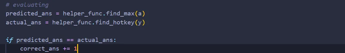
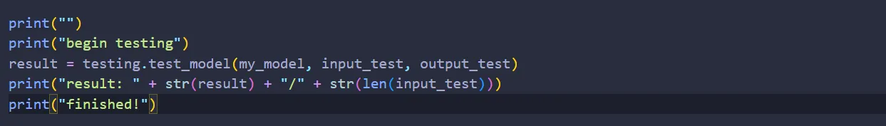
Finally, we return the correct_ans. Here’s the completed code:
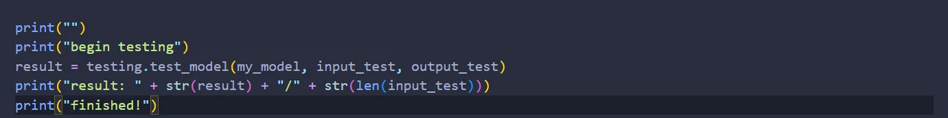
And we’re done! All that’s left to do is call the function to test our network:
Here’s the completed code of MLP.py:
And that’s it! You’ve just built your own neural network from scratch!