What’s this blog about?
This is the first part of Creating Neural Networks: Concepts, Math, and Code, where I will be talking about the theoretical concept of a neural network. Part II will implement the theory discussed here into the code.
BTW, all the codes are available on my GitHub repo.
Lastly, this is a blog I wrote at Medium.com back in 2023 when my writing skills were worse; so you may find it too wordy.
When I first learn neural networks, I was introduced to a machine learning library (ML) called TensorFlow. In my opinion, TensorFlow is a good library — too good, in fact, that they abstract all the complicated implementations away. Because of this, I tried to learn neural networks from various sources such as 3Blue1Brown and Michael Nielsen’s online book. In the end, I was able to create my own simple neural networks from scratch.
Now, I will share what I learned and guide you on how you can create your own neural networks from scratch as well, using only NumPy module to handle linear algebra operations.
Intuition
What does neural networks do, actually?
Well, consider this scenario: let’s say you want to go to a theme park. Before you go, there are three factors that you would like to consider: Is it sunny today? Is there any discount? Will your girl/boyfriend come?
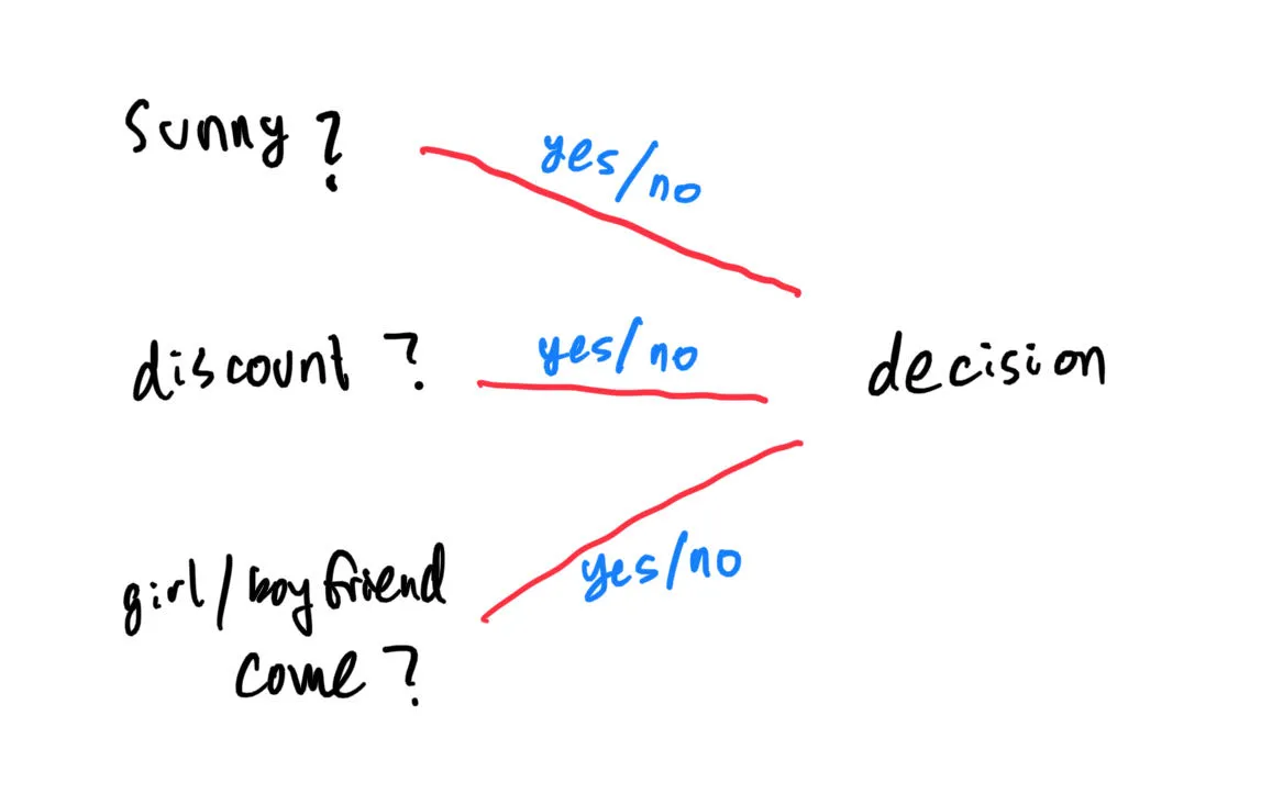
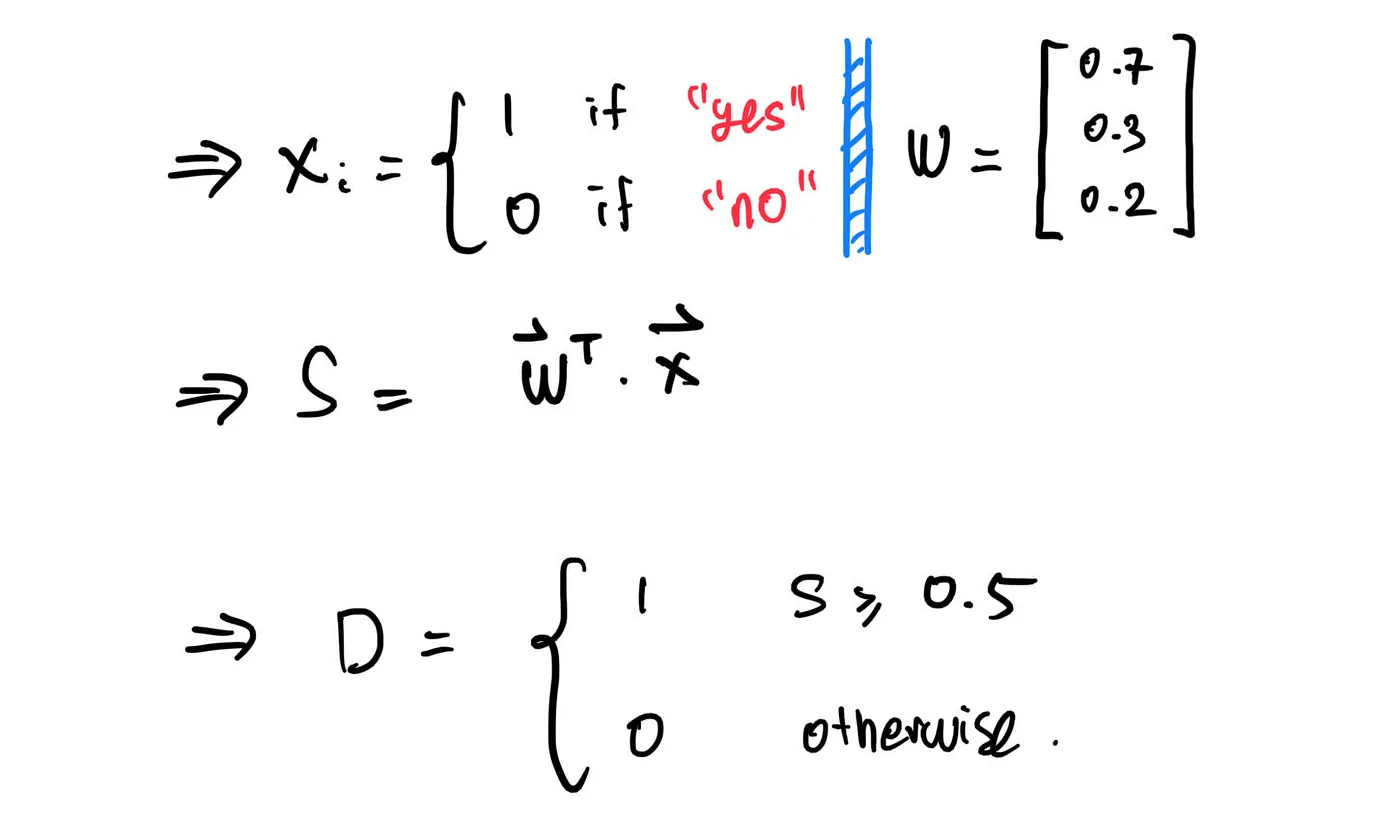
If the answer to all three of them are “yes”, you are likely to go to the theme park. However, if only one of them is a “yes”, then you probably won’t go to the theme park. Here, we can say that if “decision” has less than 2 “yeses”, then you won’t go to the theme park. Mathematically, we can express it as:
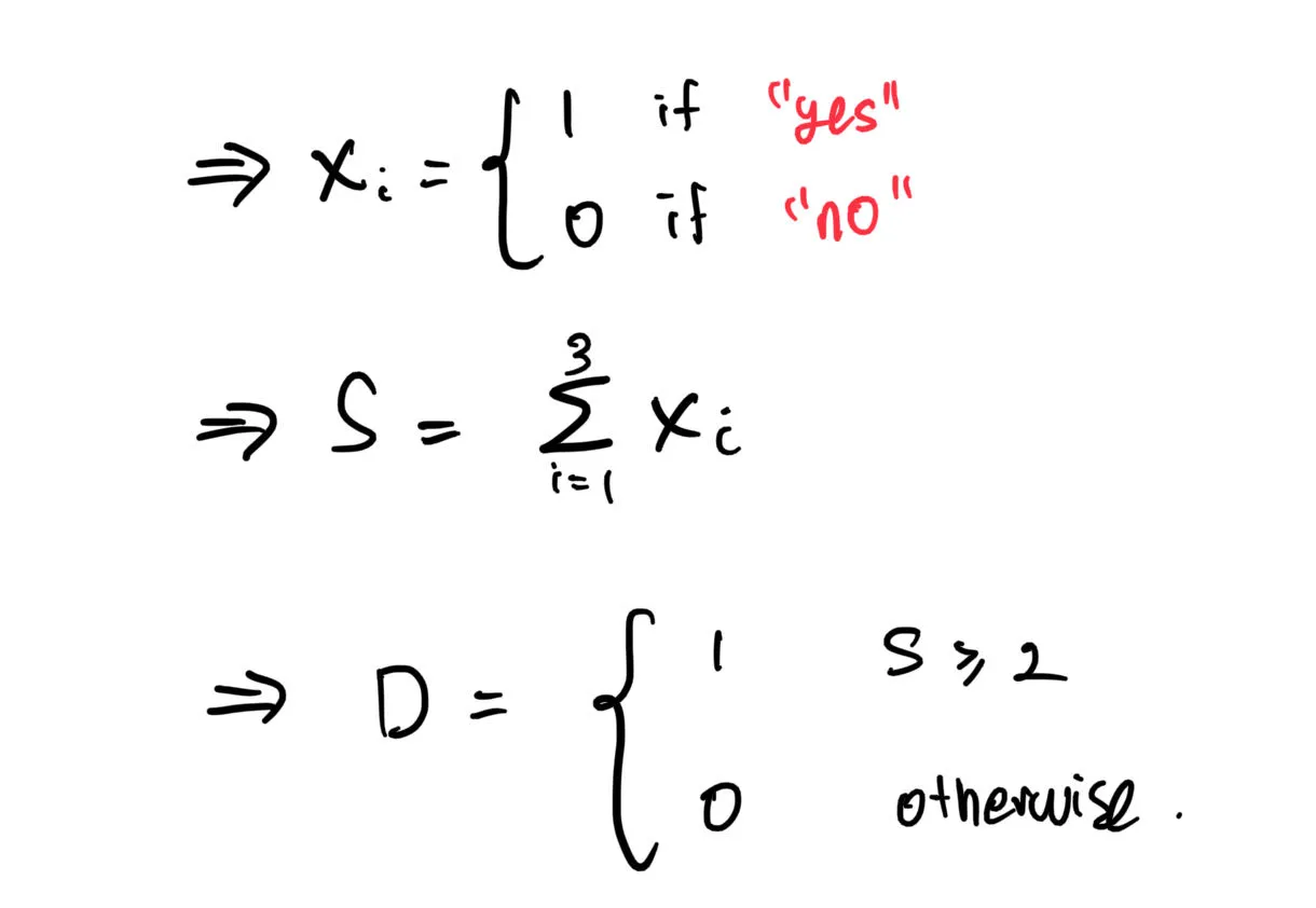
Where the vector X represents the factors (sunny, discount, girl/boyfriend go).
Maybe there are other factors you consider to be more important. For example, if your girl/boyfriend won’t come, you are still willing to go to the theme park alone. If, however, it happens to rain, then you decide to not go, even if the theme park offers discount and your girl/boyfriend is willing to go. In this case, we are adding weights to each factor.
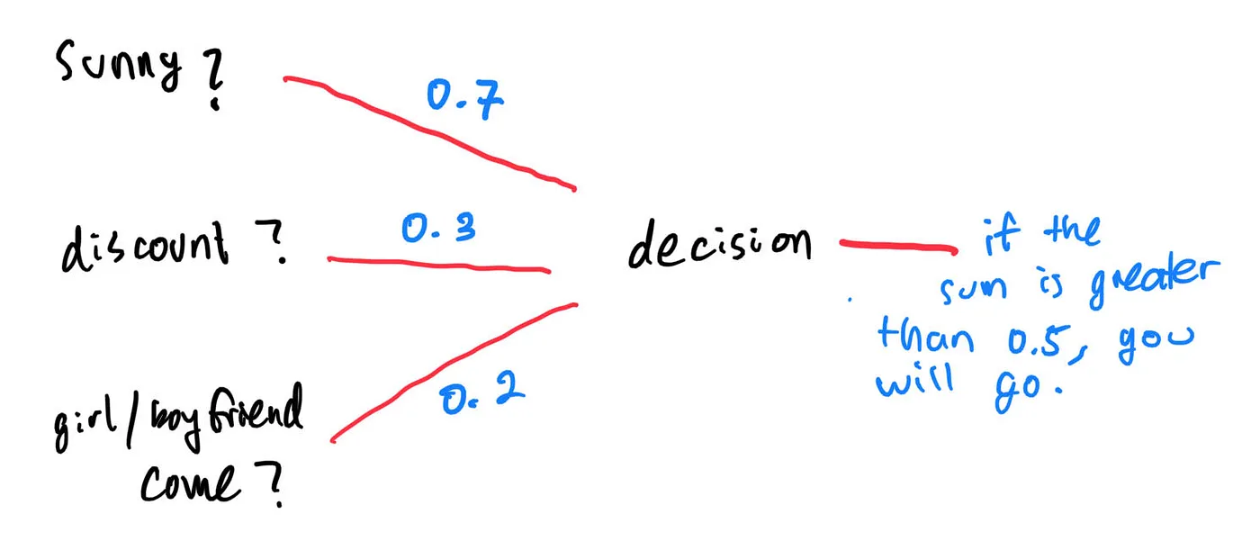
The above diagram can be expressed as:
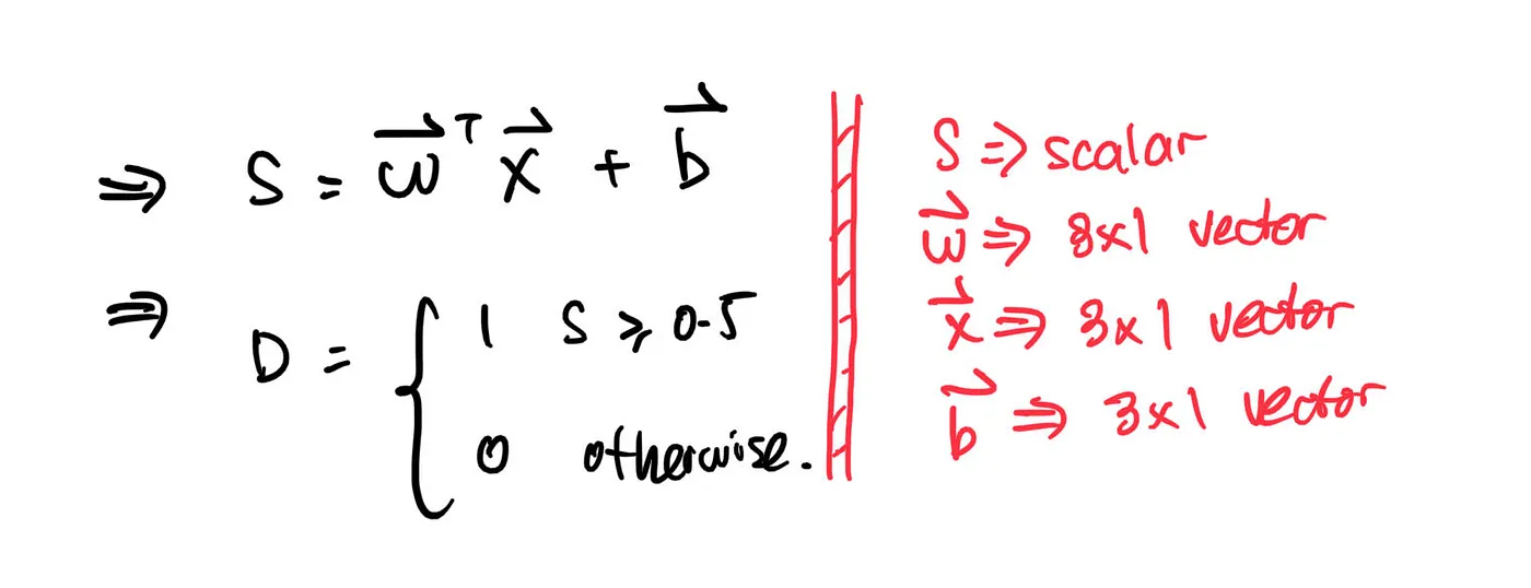
Maybe you reallyyy want to go to the theme park, since you want to ride a roller coaster so badly. In that case, you can add some fixed number to the sum, so it is more likely for the “decision” to output a number greater than 0,5. We call this fixed number as “bias”.
Mathematically, the decision can be expressed as:
In a nutshell, this is what neural networks do! The difference is, actual neural networks are more complex.
Recognizing Handwritten Digits
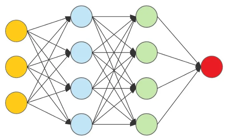
images contain pixels, and each pixels can be represented by a number. More importantly, when building a neural network to recognize handwritten digits, each pixels can be thought of as a “factor” used in “deciding” what number is written on that image.
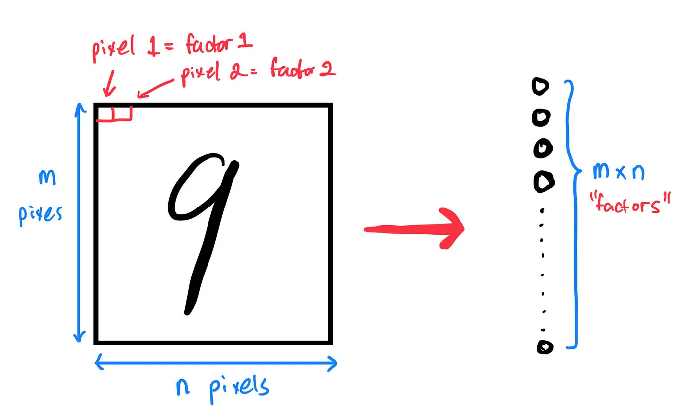
These so-called “factors” will then be given weights to them, before being fed into another layer of “sub-factors”, and the process repeats until we reach the final layer, where a “decision” is made on what digit is written on the image. By the way, all the circles representing “factors” & “sub-factors” are known as nodes.
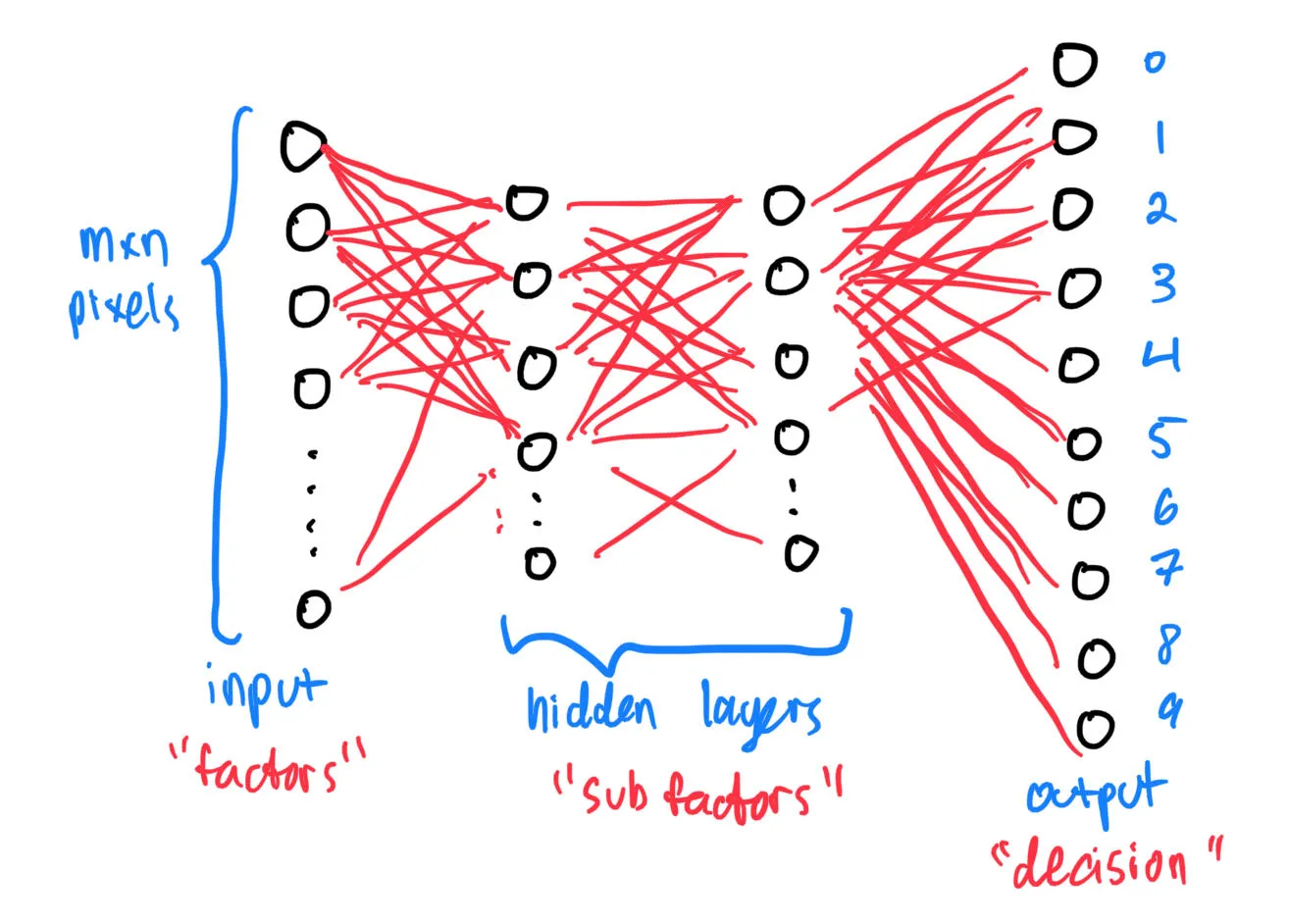
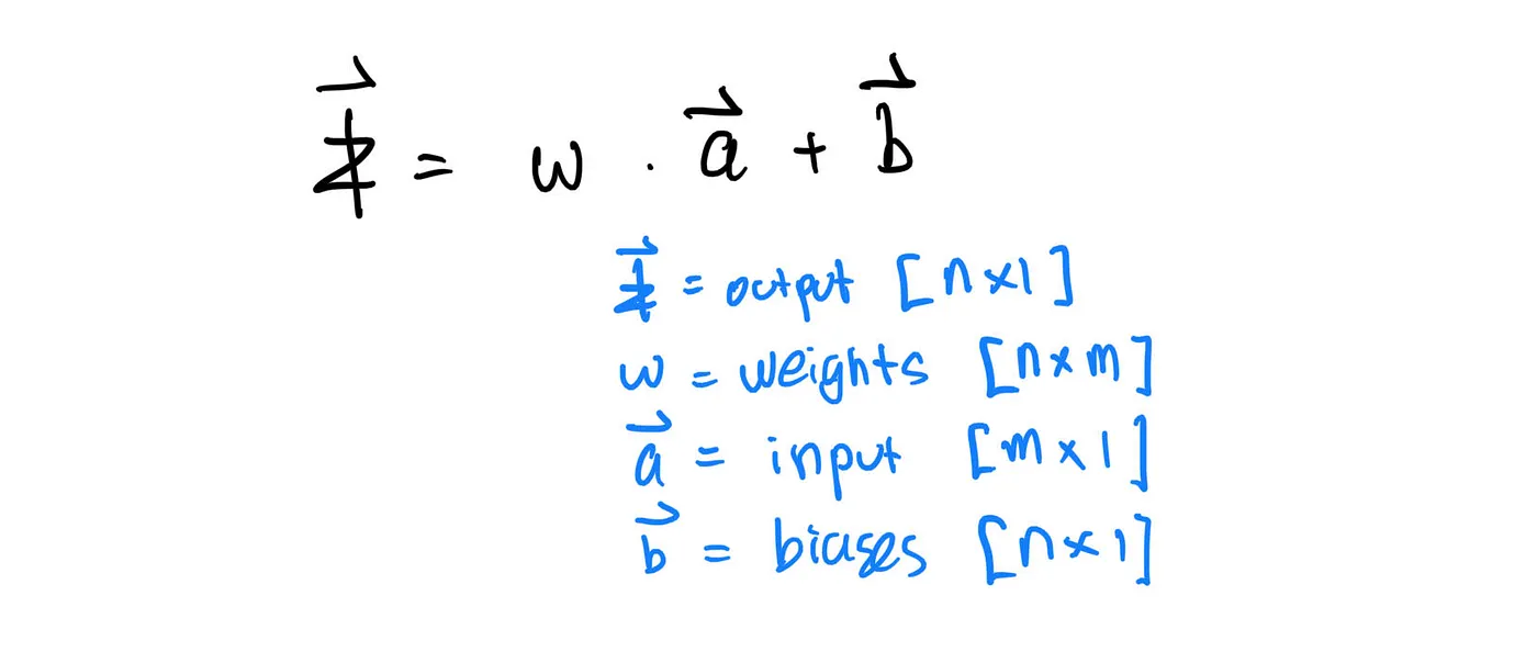
The layers above are known as dense or fully connected layers. Mathematically, the output z of a given layer is given as:
In practice, we implement the so-called “activation functions” to add non-linearity to the output of a given layer. So, if we chain an activation layer after a dense layer, the output then becomes:

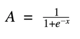
There are various kinds of activation function. Sigmoid is a common example:
Here, after passing through all the layers, the neural net decides what number it thinks the image represents by taking the largest value among the output nodes.
Learning
Initially, we set all the weights and biases for each layers randomly. Obviously, the network will be really bad at predicting what number is being written on the image! For this, the network needs to be trained. But how?
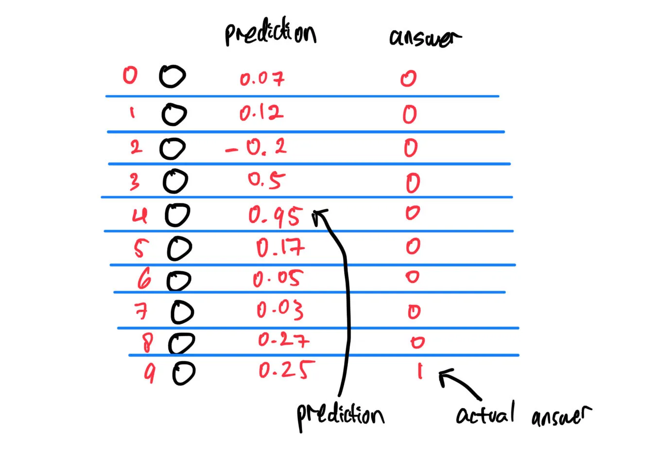
For each prediction made by the network, we tell the network what the actual answer is. For example, let’s say that the network predicts that a given handwritten digit is a “4”, while in reality the correct answer is “9”:
Given these information, we can tell the network how good or bad its prediction is by defining an error function as follows:
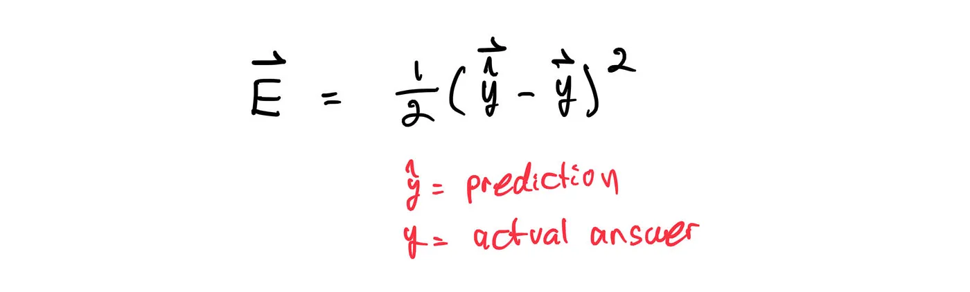
Since there are 10 nodes at the output layer, the error function we are dealing with lies in 11-D (10 inputs, 1 output). To simplify things (because my low-dimension brain can’t imagine 11-D space), let’s assume that there is only 1 node at the output layer. We can graph our error function as:
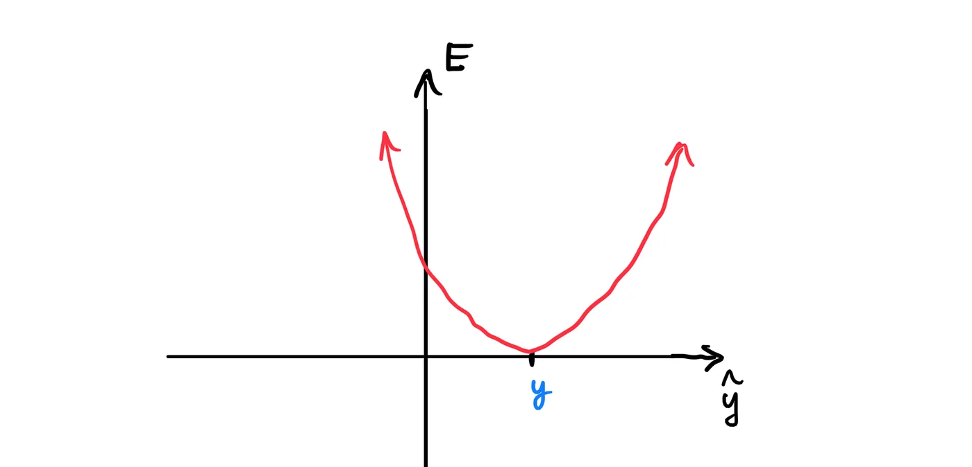
From the graph, we can see that our error is minimized when y-hat equals y. So, our goal in training the network is to tune the weights & biases of the network such that the vector y-hat equals or approximates the vector y for any given input vector of size m*n x 1.
Another way to think of it is, imagine the error function as some kind of valley. Our goal is to get to the minimum point of the valley; that is, the bottom of the valley.
Numerical Methods
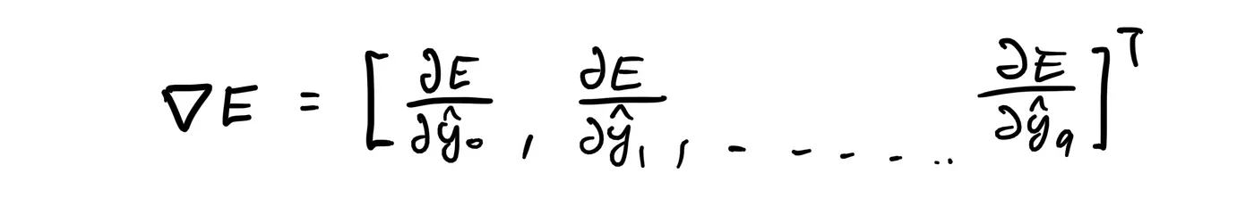
Going back to 11-D, one way to get to the bottom of the valley is by using numerical methods. In this case, it is analogous to taking steps in the direction towards the bottom of the valley. Of course, we want to pick the direction with the steepest slope, so we reach the bottom faster. Those studying Multivariable Calculus can already tell that the direction we want is given by:
so, if our current position is y-hat, then we want to subtract it by nabla E multiplied by some learning rate gamma.

And we repeat in each step until we reach the bottom (or close to the bottom) of the valley. This is known as Gradient Descent.
Another method in traversing down the hill is known as Stochastic Gradient Descent. It has the same principle with gradient descent, except that in SGD, we let the network make multiple predictions, then average the error. The averaged error is the one that we use to determine the direction of greatest slope downhill.
Backpropagation
With gradient descent, the output layer can iteratively learn to minimize its error. However, what about the previous layers?
Let’s start from the layer right before the output layer, the second last layer. Given the direction of greatest slope downhill for the output layer, we can find the direction of greatest slope downhill for the second last layer using the chain rule:
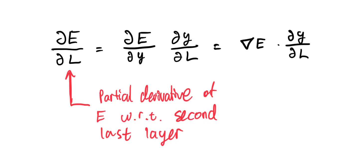
To generalize, for any two consequtive layers a and a+1:

So, if we know the partial derivative of the error with respect to a given layer, we then can easily find the partial derivative of the error with respect to the layer before. Using this idea, we can iteratively go backwards until gradient descent (or SGD) has been performed on all layers (Hence backpropagation!).
You may wonder, how does the layer a relates to the layer a+1? Well, it depends on what kind of layer L is, and will be covered in Part II.